Signal Filtering

Introduction

As you may have noted from previous lessons, sometimes the sensor reading function returns strange values. For example, an ultrasonic range finder reads (erroneous) really large distances from time to time, even when there is a near object in front of it. In this lesson we will learn some simple techniques that will help us to reduce the effects of the noise and false readings from the robot’s sensors. Also, we will introduce here some basic concepts about the analog to digital signal conversions used in Sparki.  

What You’ll Need

• A Sparki.

 

Analog to Digital Signal Conversions

Before start to work with Sparki’s sensors, let’s see some basic concepts about the way that our small robot receives information from the external world. As you may know, Sparki’s brain is a small digital microcontroller (MCU), specifically an Atmel ATMega32U4. And by digital we mean that in its inside, it deals with digital signals composed of only ones and zeros (where a digital one is represented by 5 Volts and an digital zero is represented by 0 Volts). Thus, in order to work with analog signals, which in our context are basically signals that can vary from 0 to 5 V in a continuous way, Sparki’s MCU has to translate them into ones and zeros. There are several techniques to do this conversion and Sparki’s MCU includes from factory an Analog to Digital Coverter (ADC). Let’s see first how it works in a generic way, so after having a basic understanding, we can deal with the specific details of our ADC. Please take a look to the following figure:

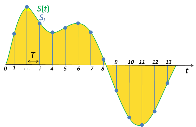
Original image from Wikimedia Commons.

There, the green line represents the continuous analog signal, while the yellow surface is the area under the curve. As our small MCU can’t do much with that curve, the ADC enters in scene, taking samples of only a subset of the signal’s points (or values), and expressing each of these values with a binary number (an integer). As you may have guessed, the  blue points in the previous figure are representing the sampled points. So here, a few questions appear. For example: how many samples should the ADC take in order to represent the original signal? That’s a good question, so let’s talk about it a bit more.  

ADC Sampling Rate

We are not selecting the ADC hardware here. In fact fact we already have the ADCs in our Sparki’s MCU. And each ADC has some specifications given by the manufacturer. So, the question about how many samples should we take, could be also asked as how many samples can we take with our current ADC hardware. And the samples that our ADC can take per second is a feature called Sampling Rate. In general, higher sampling rates will let us to convert faster changing analog signals. Think about it: if a signal changes a lot between 2 sample points, the ADC will loose all that intermediate information. On the other hand, if we need to store the signal’s digitized representation, more sampled points per second will result in the need of more storage space. Thus, a higher sampling rate is not always necessary. In fact, most modern ADCs has a configurable sampling rate (if you are curious about the low level details of the ADC configuration, you can take a look to the ATMega32U4 complete datasheet’s Analog to Digital Converter chapter). So, to help answering our original question there is a theorem (surprised?), called Nyquist–Shannon sampling theorem. Although it’s a bit complex, the final conclusion from that theorem, in everyday language is that our sampling frequency should be “twice the highest frequency of interest”. Sparki’s ADC has a maximum sampling rate of 15 KSPS (Kilo Samples Per Second), often called a 15 KHz sample frequency (being the KSPS a much more accurate term for describing ADC sample rates). So, make your conclusions about the maximum frequency of the signal that can be converted with this hardware. A note here: Although the sampling rate in theory should be higher, the specific ATMega32U4 ADC works really better with frequencies under 4 KHz, due to the way in which it’s gain stage has been designed.  Happily, this is well enough for most of our needs using Sparki’s sensors.  

ADC Resolution

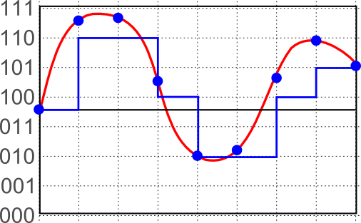
Another important question about the conversion of a signal to the digital domain is the size of the numbers used to store each sampled point. For example, if we use just 8 bits to store a sampled value, we can represent it with only 256 different numbers. So, any point between the possible representations will be rounded to an approximate value. In the following figure, for example, we are showing an ADC technique (with 3 bits of resolution) where each sampled value (blue points) from the original signal (red curve) is mapped to a binary number below the sampled point, resulting in the blue signal. We can see clearly that the approximation is not really good with just 3 bits in this case: The quantity of bits used to store the sampled values is called the resolution of the ADC. As with the sample rate, a higher resolution means in general a better representation of the signal, but it also takes more memory space when storing it. And will need more processing power if we want to work mathematically with that signal. Sparki’s ADC features a 10 bits (maximum) resolution. This means that the analogRead function used inside the libraries for sensors like the Infrared Reflectance Sensors, or the Light Sensors can return numbers between 0 and 1023 (since 2^10 = 1024). Again, that’s good enough, as you may have seen in the previous lessons when working with Sparki’s sensors!  

Averaging Ultrasonic Range Finder Readings

Now that we have learned a few things about signal conversions, let’s start to work with real signals from the Sparki sensors. If you try the following code snippet, adapted from the Ultrasonic Ranger Finder page code, you will note that if you move your hand oscillating quickly towards and from the robot, you may see some sensor readings which are clearly false readings (with numbers like 150 cm, for example):

Some of these readings could even be true, but we are not interested in them, since they may be the result of a temporary event that should not affect our robot’s behavior (for example something passed fast in front of the robot, thus not being a real obstacle if the robot is moving forward). So, to improve the confidence in our sensor readings, and if the speed of these readings is not critical, we can always apply a simple technique: the average. This way, instead of just printing the result of one single reading, we will take the value of 3 of them (this number is arbitrary, of course, and should be adjusted to our specific needs) and calculate the average (or arithmetic mean). This is the sum of all the read values, divided by the quantity of readings (or signal samples). Take a look to the following code:

If you even try to quit quickly your hand from the front of the sensor, you will note that the readings do not “move” a lot from one to the other. Of course, this is also done at the cost of measuring speed (or sample rate as we have seen above). As you can see in the previous code, all the work is done in the average function. This function receives the desired number of sensor readings as a parameter. We defined this parameter as an unsigned integer number (called numberOfReadings). It’s unsigned, since it does not make sense to have a negative number of readings. The core of the average function is a for cycle, which iterates “numberOfReadings” times, adding the new sensor reading value to the previous (accumulated) values: Finally, the function just returns the quotient between the sum of the readings and the number of readings. Before moving on, you can play a bit with different values for the numberOfReadings parameter…  

A Generic Average Function

But what if we want to apply the average function to other sensors? Sparki has plenty of sensors, and calculating the arithmetic mean of their readings could be useful not just for the ultrasonic distance ranger, but for all of them. Even digital readings could be averaged (try it!). So, why not write a generic average function that we can use with any of these useful sensors? Let’s take a look to the following code:

And now let’s analyse the previous code a bit deeper. Of course, the most important part here is the average function: But unlike our previous average version, which was limited to work only with the ultrasonic distance ranger, this new function has some modifications which convert it into a generic function. Now, it can calculate the average of an arbitrary number of readings (the parameter numberOfReadings) for any Sparky sensor. To accomplish that, we have introduced two changes to the code. The first is quite simple: the fixed delay was changed by a variable delay, adding a new parameter called readingsDelay. This way, the previous delay(20) is now the following line: This is important because different sensors may need different delays, or no delay at all (that’s why we added the if statement there, so if readingsDelay has a value of zero, the delay() function is not even called). The second change is a bit more complex, but easy to understand too. As you can see in the code, the call to the sparki.ping() function was replaced by a call to something called callBack(). So, what’s this? A callback function is a function that we can pass as a parameter to another function, making it possible for this last one to call it. This enables the function to call different (callback) functions in different situations. The basic idea here is that we define new functions to read sensors, and then we pass the function for each sensor to our average function as a parameter, as you can see in our code’s loop: There, average is called first with pingCallBack as its first parameter, then with accelXCallBack, and so on. But if you take a look to the definitions of pingCallBack and the other functions, they are just standard functions with nothing special, except for the fact that all of them has the same signature, which just means that they return the same kind of thing (a float in our case) and receives exactly the same kind of parameters (nothing in our functions): So if we take a look again to the definition of the new average function, the first parameter just specifies the format of the functions that average is expecting to receive: Where float is the return type, and (*callBack) is the name to be used inside the average function when we call it. Please take into account that it may be any valid C/C++ function name and we just used callBack because it liked to us, nothing else. But it’s important to enclose it with parenthesis and to add the “*” before the name, to indicate that we are passing a pointer to a function (please don’t worry if you don’t understand the pointer concept right now, since it’s not really important to understand this lesson). Finally, the “(void)” construction there indicates that the callback function itself will not receive parameters. Again, the parenthesis there are important. Inside average, the callback function will be called by it’s name, just as any other function call. In our case, se add the result returned by callBack() to the result variable:  

More Advanced Filters

When processing a signal, filters are the processes (and/or devices) that remove unwanted features or components from that signal. According to the application on which you may be working on, there are plenty of other filters that may be useful to work with Sparki’s sensors. Some of them could be the low-pass, the high-pass, the median filter, etc.. We are not going to implement them here, but you can take this lesson as a starting point to experiment and play with these kind of algorithms. And if you want a more advanced reading, take a look to this Digital Signal Processing free book.  

Extra Activities and Related Lessons

Now that we know a bit more about Sparki’s sensors, its ADC and some simple ways to improve sensor readings reliability, why not apply these ideas to some of the previous lessons? Here is a small list of related lessons which may be improved, or which you can use to experiment a bit:

• Wall Avoidance
• Theremin
• Making Music with the Accelerometer
• Maze Solving